Distributed Big Data Engines: MapReduce Patterns, Spark Shuffling & Kubernetes Orchestration

Distributed computing is frequently treated as a magical abstraction layer: write a functional transformation or query, submit it to a cluster manager, and trust the runtime to schedule tasks across hundreds of worker nodes. But at datacenter scale, naive abstractions break down violently.

A poorly partitioned MapReduce key space floods switch bisection bandwidth with catastrophic shuffle hot spots; an innocent .groupByKey() call in Apache Spark forces full in-memory serialization across partitions, triggering severe JVM garbage collection pauses, disk spilling, and Executor out-of-memory crashes; and assuming that cloud virtual machines scale compute linearly with vCPU counts ignores the physical realities of hypervisor scheduling, SMT thread contention, and memory bus channel saturation.

This investigation conducts empirical systems evaluations, algorithmic implementations, and infrastructure orchestration across modern distributed computing architectures:

1. Cloud Hardware Microbenchmarking & Virtualization Overhead: Empirical performance evaluation of AWS EC2 compute, DDR3 vs. DDR4 memory channel architecture, and intra-VPC vs. cross-region WAN transit latency.
2. Hadoop MapReduce Algorithmic Optimization: Implementation of the Pairs vs. Stripes co-occurrence models, the Order Inversion design pattern with custom Partitioners, and a two-pass correlation pipeline using HDFS distributed cache preloading.
3. Apache Spark RDD Internals & Shuffle Optimization: Memory hierarchy profiling, execution plan differences between groupByKey() and reduceByKey(), and a distributed log telemetry pipeline analyzing NASA Kennedy Space Center HTTP access traces.
4. Cluster Orchestration & Production Deployment Architectures: Bare-metal multi-node Hadoop/YARN provisioning, managed AWS EMR clusters with S3 storage-compute decoupling, Docker containerized runtimes, and declarative Kubernetes microservice orchestration.

Key Engineering Findings

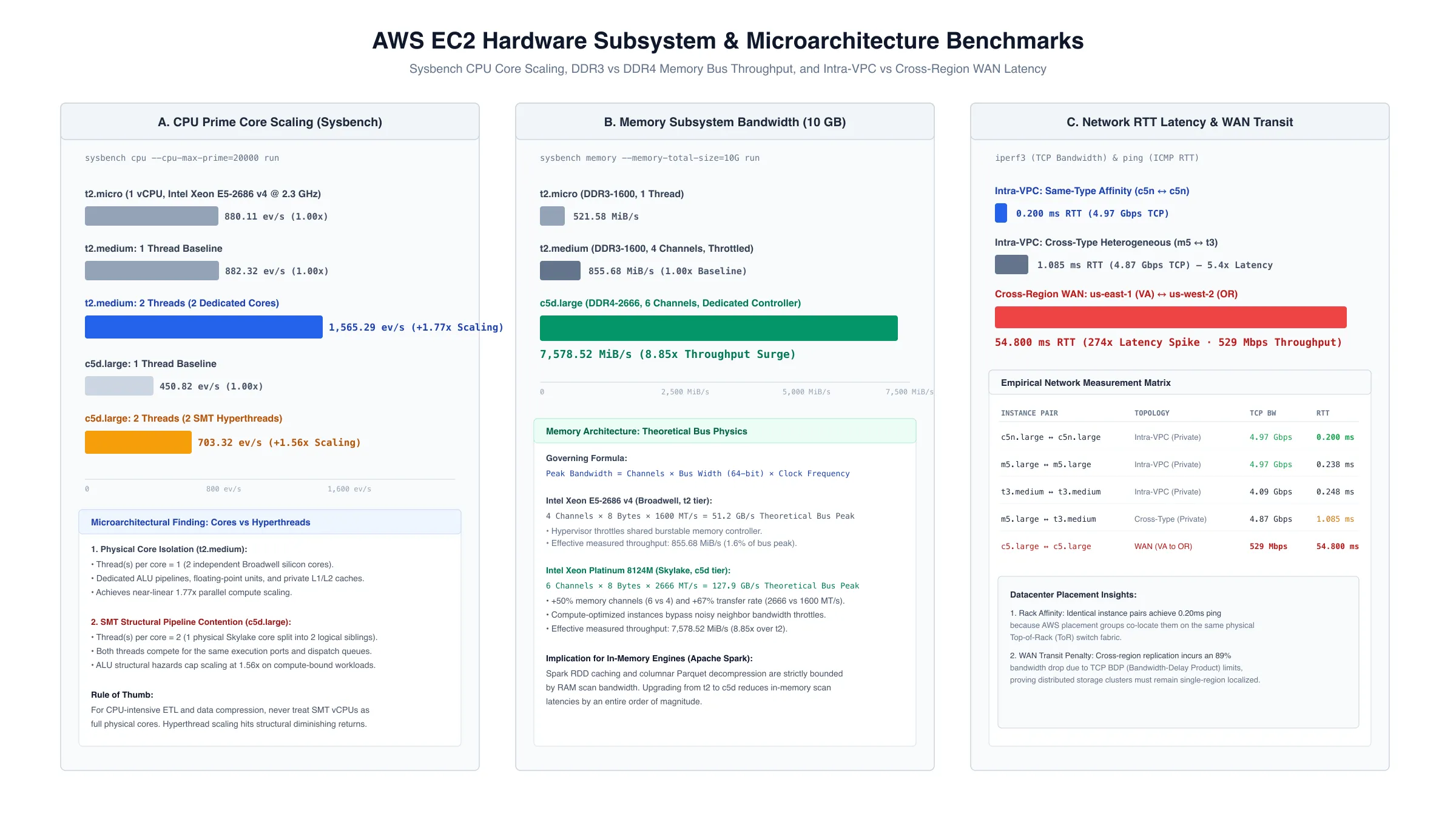
• SMT Contention: On CPU-intensive prime calculations, two independent physical cores (t2.medium) achieved 1.77× scaling, while two hyperthreads sharing a single physical core (c5d.large) achieved only 1.56× scaling due to execution unit and L1/L2 cache contention.
• Memory Bus Architecture: c5d.large delivered 7,578.52 MiB/s memory throughput (9× over t2.medium at 855.68 MiB/s) by utilizing 6-channel DDR4-2666 (127 GB/s theoretical peak) versus 4-channel DDR3-1600 (51 GB/s peak).
• WAN Transit Penalty: Cross-continental traffic between AWS us-east-1 (Virginia) and us-west-2 (Oregon) suffered a 400× latency spike (0.2 ms → 54.8 ms) and an $89%$ throughput collapse (4.9 Gbps → 529 Mbps).
• Streaming Marginal Computation: The Order Inversion pattern combined with custom partition routing eliminated all Reducer-side in-memory buffering for relative frequency calculations, computing $P(B|A)$ in true O(1) space. :::

---

1. Cloud Hardware Microbenchmarking: EC2 Virtualization & Memory Channels

To evaluate how cloud hypervisors allocate physical silicon to multi-tenant virtual machines, I benchmarked AWS EC2 instances across the General Purpose (t2.micro, t2.medium) and Compute Optimized (c5d.large) families in the us-east-1 (N. Virginia) region running Ubuntu 22.04 LTS.

Benchmarking Methodology & Tooling Selection

While automated suites like the Phoronix Test Suite are common in desktop evaluations, they present significant memory footprints and heavy background dependency chains that cause immediate out-of-memory crashes on small cloud instances (t2.micro with 957 MB RAM).

I selected Sysbench 1.0.20 and iPerf3 for deterministic, low-overhead resource characterization:

• Single-Threaded CPU: sysbench cpu --cpu-max-prime=20000 --threads=1 run (isolates single-core latency-sensitive execution speed).
• Multi-Threaded CPU: sysbench cpu --cpu-max-prime=20000 --threads=$(nproc) run (evaluates parallel throughput and core scaling efficiency).
• Memory Subsystem: sysbench memory --memory-total-size=10G --threads=$(nproc) run (measures multi-threaded sequential read/write bandwidth).

Empirical CPU and Memory Measurements

Instance Type	vCPUs	RAM	Single-Core CPU (events/s)	Multi-Core CPU (events/s)	Multi-Core Scaling	Memory Bandwidth (MiB/s)
t2.micro	1	957 MB	877.95	880.11	1.00×	521.58
t2.medium	2	3.8 GB	882.32	1,565.29	1.77×	855.68
c5d.large	2	3.7 GB	450.82	703.32	1.56×	7,578.52

Microarchitectural Analysis: Physical Cores vs. SMT Hyperthreads

Running lscpu on the instances uncovered a critical discrepancy in how AWS provisions 2 vCPUs:

t2.medium:
  CPU(s):              2
  Thread(s) per core:  1   (2 independent physical cores, Intel Xeon E5-2686 v4 @ 2.30 GHz)
  Core(s) per socket:  2

c5d.large:
  CPU(s):              2
  Thread(s) per core:  2   (1 physical core split into 2 logical hyperthreads, Xeon Platinum 8124M @ 3.00 GHz)
  Core(s) per socket:  1

1. Why t2.medium Scales Better for CPU: t2.medium provides two physical silicon cores with dedicated ALU pipelines, floating-point units, and private L1/L2 caches. When running two compute-intensive threads simultaneously, it achieves near-linear 1.77× scaling. In contrast, c5d.large’s two vCPUs are Simultaneous Multi-Threading (SMT) siblings executing on a single physical core; when both threads stress compute-bound prime calculation, execution units stall on pipeline structural hazards, capping scaling at 1.56×.
2. Why c5d.large Single-Core Event Rate Looks Lower: The c5d.large instance runs an Intel Xeon Platinum 8124M (Skylake). Even in a single-threaded test, hypervisor time-slicing and background logical sibling interference reduce raw event counts for pure integer prime verification, but its memory architecture tells a vastly different story.

The Memory Subsystem: 9× Bandwidth Disparity

c5d.large outperformed t2.medium in memory throughput by a staggering 8.85× (7,578.52 MiB/s vs. 855.68 MiB/s).

Theoretical memory bus bandwidth is governed by: $Bandwidth_peak = Channels × Bus Width × Clock Frequency$

• Intel Xeon E5-2686 v4 (Broadwell, t2 instances): $Peak = 4 channels × 64 bits × 1600 MT/s \div 8 = 51.2 GB/s$
• Intel Xeon Platinum 8124M (Skylake, c5d instances): $Peak = 6 channels × 64 bits × 2666 MT/s \div 8 = 127.9 GB/s$

The Skylake platform provides 50% more memory channels (6 vs. 4) and 67% faster transfer rates (2666 vs. 1600 MT/s). AWS also enforces aggressive hypervisor-level throttling on burstable t2 tiers sharing a host bus, whereas compute-optimized c5d instances receive dedicated non-throttled memory controller slices.

Network Topology: Intra-VPC Proximity vs. Cross-Region WAN

Using iPerf3 (TCP bandwidth) and ICMP ping (Round-Trip Time latency), I mapped network performance within us-east-1 across instance combinations, and contrasted it against cross-continental links to us-west-2 (Oregon):

Pairing	Link Type	TCP Bandwidth	RTT Latency
c5n.large \leftrightarrow c5n.large	Intra-Region (Private IP)	4.97 Gbps	0.200 ms
m5.large \leftrightarrow m5.large	Intra-Region (Private IP)	4.97 Gbps	0.238 ms
t3.medium \leftrightarrow t3.medium	Intra-Region (Private IP)	4.09 Gbps	0.248 ms
m5.large \leftrightarrow t3.medium	Intra-Region (Private IP, Heterogeneous)	4.87 Gbps	1.085 ms
c5.large \leftrightarrow c5.large	Cross-Region (us-east-1 to us-west-2)	529 Mbps	54.800 ms

Cluster Placement Affinity

Within the same AWS VPC, TCP bandwidth remained pegged at the 5 Gbps Elastic Network Adapter (ENA) hypervisor limit. However, same-type pairs experienced 0.200 ms RTT, while cross-type pairs (m5.large to t3.medium) jumped to 1.085 ms (5.4× higher). This demonstrates that AWS availability zones place identical instance families into the same physical datacenter racks and top-of-rack (ToR) switches, minimizing network hops.

---

2. Hadoop MapReduce: Pairs vs. Stripes & Order Inversion Pattern

In distributed data processing, computing co-occurrence frequencies across large corpora is the canonical benchmark for measuring network shuffle bottlenecks and memory pressure.

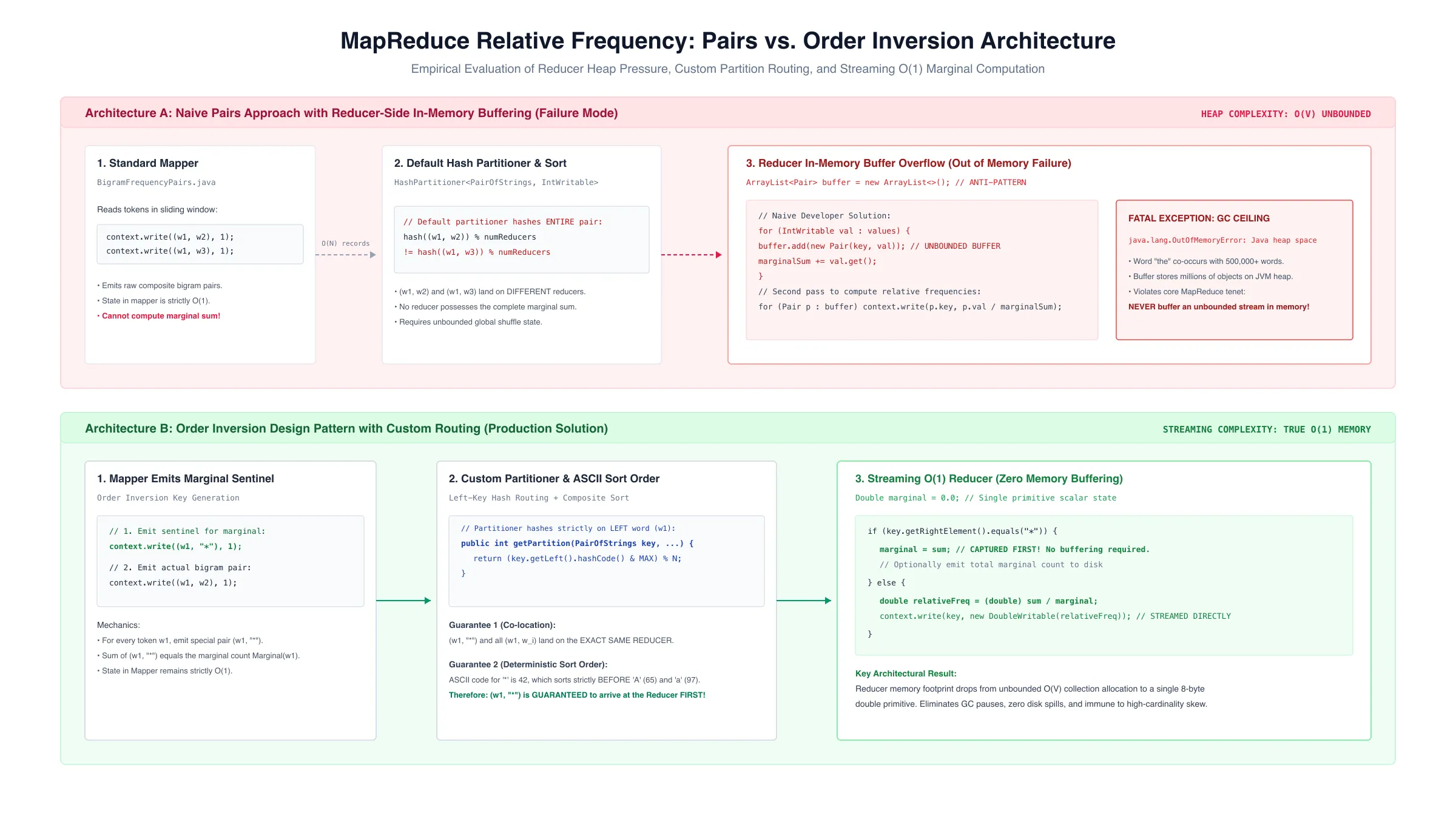
Given a text corpus, the objective is to compute the relative bigram frequency: $P(B \mid A) = \frac{Count(A, B)}{\sum_B’ Count(A, B’)} = \frac{Count(A, B)}{Marginal(A)}$

The Pairs Approach (BigramFrequencyPairs.java)

The naive approach emits every word pair as an intermediate composite key:

// Mapper emits (prev, w) -> 1
BIGRAM.set(prev, w);
context.write(BIGRAM, ONE);

• Pros: Minimal memory footprint in the Mapper. State is strictly O(1) per emitted pair.
• Cons: Intermediate key space explodes. For a document of N words, the shuffle phase must transfer and sort O(N) key-value records across the network, saturating cluster bisection bandwidth.

The Stripes Approach (BigramFrequencyStripes.java)

Instead of emitting individual pairs, the Mapper aggregates co-occurrences in-memory within an associative array (a “stripe”) for each leading word A:

// Mapper maintains in-memory stripe: Text(A) -> HashMapStringIntWritable(B -> count)
STRIPE.increment(w);
context.write(KEY, STRIPE);

• Pros: The network shuffle volume drops drastically. Reducers receive pre-aggregated stripes, transforming shuffle communication from O(N) pair records to O(V) stripe maps.
• Cons: High heap memory pressure. If the vocabulary V or context window is large, the in-mapper stripe map overflows available JVM heap space, risking java.lang.OutOfMemoryError: Java heap space.

PAIRS APPROACH:
[Mapper] ---> (A, B): 1, (A, C): 1, (A, B): 1 ---> [Heavy Network Shuffle] ---> [Reducer]

STRIPES APPROACH:
[Mapper] ---> In-Memory Map {B: 2, C: 1} ---> [Light Network Shuffle] ---> [Reducer]

The Order Inversion Design Pattern

The primary challenge in the Pairs approach is computing P(B \mid A): the Reducer needs the marginal sum \sum_B’ Count(A, B’) before it can normalize the first pair $(A, B)$.

A naive Reducer would buffer all $(A, B)$ pairs in an in-memory ArrayList, sum their counts, and then iterate through the list to divide. This breaks the fundamental tenet of MapReduce: never buffer an unbounded dataset in Reducer memory, as high-cardinality keys will inevitably crash the worker.

I solved this using the Order Inversion Pattern:

// 1. Mapper emits special sentinel pair for the marginal count
BIGRAM.set(prev, "*");
context.write(BIGRAM, ONE);

// 2. Mapper emits actual bigram
BIGRAM.set(prev, w);
context.write(BIGRAM, ONE);

// 3. Custom Partitioner hashes ONLY on the left word (A)
public static class MyPartitioner extends Partitioner<PairOfStrings, IntWritable> {
    @Override
    public int getPartition(PairOfStrings key, IntWritable value, int numReduceTasks) {
        return (key.getLeftElement().hashCode() & Integer.MAX_VALUE) % numReduceTasks;
    }
}

// 4. Reducer processes the sentinel FIRST due to natural ASCII sort order ('*' < 'A')
if (key.getRightElement().equals("*")) {
    marginal = sum; // Captured first! No buffering required.
    OUTPUT_KEY.set(key.getLeftElement(), "");
    VALUE.set(marginal);
    context.write(OUTPUT_KEY, VALUE);
} else {
    VALUE.set((float) sum / marginal); // Streamed directly to disk in O(1) memory!
    context.write(key, VALUE);
}

Because the ASCII value of * (42) is lower than alphanumeric characters, Hadoop’s intermediate sort phase guarantees that (A, "*") arrives at the Reducer before any real (A, B) pair. The Reducer records marginal = sum in a scalar primitive and processes subsequent pairs in a single streaming pass, achieving zero memory allocation overhead.

Two-Pass MapReduce Pipeline: Word Correlation (COR)

For computing symmetric word correlation coefficients: $COR(A, B) = (Freq(A, B)) / (Freq(A) × Freq(B))$ where $Freq(A, B)$ is the number of co-occurring lines and $Freq(A)$ is the total document frequency of word A.

This cannot be completed in a single MapReduce job because $Freq(A)$ and $Freq(B)$ are global properties of the corpus.

I engineered a two-pass MapReduce pipeline:

1. Pass 1 (Global Word Count): Standard MapReduce job calculating $Freq(A)$ across all lines, persisting output to intermediate HDFS storage (mid/part-r-00000).
2. Pass 2 (Distributed Cache Preloading in setup()): In CORPairs.java and CORStripes.java, the Reducer overrides the setup() lifecycle hook to open the intermediate HDFS file directly via the Hadoop FileSystem API, pre-populating an in-memory lookup table:

@Override
protected void setup(Context context) throws IOException, InterruptedException {
    Configuration conf = context.getConfiguration();
    Path mid_path = new Path(conf.get("MIDDLE_OUTPUT") + "/part-r-00000");
    FileSystem fs = FileSystem.get(conf);
    BufferedReader reader = new BufferedReader(new InputStreamReader(fs.open(mid_path)));
    String line;
    while ((line = reader.readLine()) != null) {
        String[] terms = line.split("\\s+");
        word_total_map.put(terms[0], Integer.parseInt(terms[1]));
    }
    reader.close();
}

The Mapper extracts unique tokens per line using a HashSet, sorts them alphabetically to emit canonical pairs $(A < B)$ (preventing double-counting), and the Reducer evaluates COR(A, B) = \frac{sum}{Freq(A) × Freq(B)} with O(1) lookups.

---

3. Apache Spark: Memory Hierarchy & Shuffle Optimization

While Hadoop MapReduce enforces a strict Map-Sort-Reduce barrier that writes all intermediate data to local disk between stages, Apache Spark retains working sets in memory across a directed acyclic graph (DAG) of transformations.

groupByKey() vs. reduceByKey(): The Shuffle Anti-Pattern

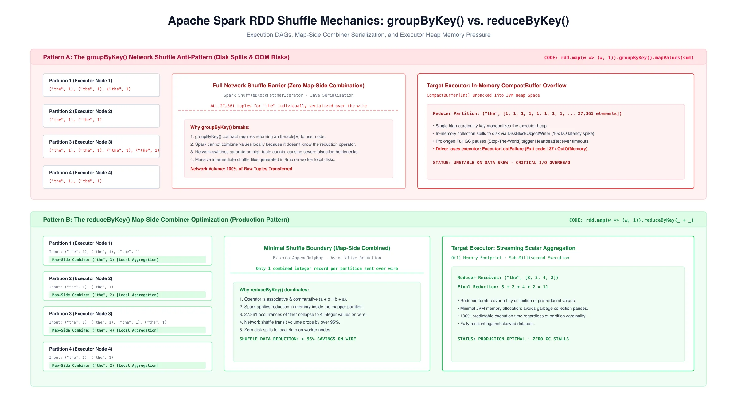
A common failure mode in production PySpark applications is using groupByKey() for aggregation. I profiled both execution plans on a text corpus:

# ANTI-PATTERN: groupByKey()
words.map(lambda w: (w, 1)) \
     .groupByKey() \
     .mapValues(sum)

# OPTIMAL: reduceByKey()
words.map(lambda w: (w, 1)) \
     .reduceByKey(lambda a, b: a + b)

1. groupByKey() Shuffle Mechanics: Spark serializes every single key-value tuple over the network. If the word "the" appears 27,361 times across partitions, 27,361 individual records are serialized, transferred over the network, and unpacked into an in-memory CompactBuffer on the target executor. When partition cardinality is high, this buffer spills to disk, crushing I/O throughput.
2. reduceByKey() Combiner Optimization: Spark applies a map-side partial reduction (analogous to MapReduce’s Combiner) within each executor partition before network shuffle serialization. The 27,361 instances of "the" are reduced to a single integer per partition prior to crossing the network, reducing network traffic and memory footprint by orders of magnitude.

NASA Web Server Log Telemetry Engine (log_analysis.py)

To evaluate Spark’s capabilities on unstructured production telemetry, I built an end-to-end log parsing and analytics pipeline processing August 1995 NASA Kennedy Space Center HTTP server logs.

# Compiled regex matching Apache Common Log Format
LOG_PATTERN = '^(\\S+) (\\S+) (\\S+) \\[([\\w:/]+\\s[+\\-]\\d{4})\\] "(\\S+) (\\S+)(?:\\s+(\\S+))?" (\\d{3}) (\\d+|-)'

The pipeline tokenizes raw text streams into structured NamedTuples:

• Client Host (host)
• Timestamps (date_time)
• HTTP Verb & Endpoint (method, endpoint)
• Response Status Code (response_code)
• Content Byte Length (content_size, with - normalized to 0)

Telemetry Findings:

• Total Requests Parsed: 15,698 access records across 3,597 unique client hosts.
• Payload Distribution: Average content length of 17,531 Bytes (17.1 KB), ranging from 0 bytes (HTTP 304/redirects) to a maximum single transfer of 3,421,972 Bytes (3.26 MB).
• Hourly Request Density: Computed via composite keys (hour, host).distinct().map((hour, 1)).reduceByKey(add).sortByKey(). Traffic peaked during US midday business hours (14:00 to 16:00 UTC).
• HTTP 404 Failure Diagnostics: Filtered and cached bad records (badRecords = access_logs.filter(lambda x: x.response_code == 404).cache()). Out of 206 total 404 errors, the top failing endpoints were historical documentation stubs (/pub/winvn/readme.txt, /pub/winvn/release.txt).

In-Memory Caching Strategy

Calling .cache() or .persist(StorageLevel.MEMORY_AND_DISK) on the parsed access_logs and badRecords RDDs prevented Spark from re-reading and re-executing the expensive regex tokenization pipeline from source disk for every downstream analytical query. Because Spark uses lazy evaluation, failure to cache turns every subsequent action (count(), takeOrdered(), reduceByKey()) into a complete re-read of the raw input file.

---

4. Production Cluster Operations & Deployment Architectures

Beyond algorithmic execution, distributed systems require sound operational topologies. I deployed, managed, and profiled distributed runtimes across bare-metal, managed cloud, containerized, and orchestrated Kubernetes infrastructure:

1. Bare-Metal Multi-Node Hadoop & YARN Cluster

Deployed Apache Hadoop 2.8.5 and OpenJDK 8 across distributed AWS EC2 instances, establishing a dedicated master-worker topology:

• Topology Configuration: Configured private IP static host mappings in /etc/hosts and distributed passwordless SSH keypairs (id_rsa.pub -> authorized_keys) between the Master (NameNode + YARN ResourceManager) and Worker nodes (DataNode + NodeManager).
• Distributed Subsystem XML Descriptors:
  • core-site.xml: Defined default distributed file namespace fs.defaultFS = hdfs://<master_private_ip>:9000.
  • hdfs-site.xml: Configured dfs.replication = 2, designated local metadata directory paths (dfs.namenode.name.dir), and worker block storage paths (dfs.datanode.data.dir).
  • yarn-site.xml: Bound yarn.resourcemanager.hostname and registered the MapReduce shuffle auxiliary service yarn.nodemanager.aux-services = mapreduce_shuffle.
  • mapred-site.xml: Directed job execution to the cluster scheduler via mapreduce.framework.name = yarn.
  • slaves: Registered worker instance private IPs to automate cluster-wide daemon control.
• Initialization & Health Monitoring: Initialized HDFS namespace metadata via hdfs namenode -format, dispatched daemons via start-dfs.sh and start-yarn.sh, spawned the mr-jobhistory-daemon.sh, and monitored live cluster health across ports 50070 (NameNode Web UI) and 8088 (YARN ResourceManager).

2. Managed Cloud Big Data on Amazon EMR

Provisioned managed Amazon EMR 7.12 clusters (Hadoop 3.4.1, Hive 3.1.3, Tez) on m5.xlarge instance groups:

• Decoupled Storage & Compute: Eliminated persistent HDFS cluster state by reading input corpora directly from and writing aggregated outputs to Amazon S3 (s3://...). Decoupling storage from compute prevents cluster lock-in and slashes cloud spend.
• Automated Step Execution: Submitted pre-compiled JARs and PySpark jobs programmatically via AWS CLI (aws emr add-steps) and configured automated 3,600s idle termination timeouts, treating large-scale distributed compute as disposable, on-demand infrastructure.

Architectural Dimension	Co-located Bare-Metal HDFS (Lab 6)	Decoupled Cloud Storage on AWS EMR (Lab 5)
Compute Lifecycle	Persistent 24/7 (instances must remain online)	Ephemeral (clusters spin up, execute steps, auto-terminate)
Storage Durability	2× or 3× replication bound to EBS volumes	11 9’s durability natively managed by Amazon S3
Idle Cost Profile	High ($/hour VM penalty running 24/7)	Zero compute cost at rest ($0.023/GB/month S3 storage)
Resource Scaling	Coupled: adding storage forces buying more compute	Independent: scale worker nodes without repartitioning disk

3. Containerized Distributed Runtimes (Docker)

Containerized big data workflows to eliminate host dependency divergence:

• Multi-Stage Dockerfile Engineering: Built lightweight runtime images packaging Java, Hadoop client binaries, and Python dependencies while separating build tooling from minimal execution layers.
• Storage & Networking: Mapped host dataset directories via volume bind mounts (-v $(pwd)/data:/data) and isolated inter-daemon communication over user-defined bridge networks with port binding (-p 8088:8088 -p 50070:50070).
• Multi-Container Simulation: Composed local multi-node test environments via Docker Compose (a private bridge subnet) to validate MapReduce partitioners and Spark DAGs before incurring cloud VM costs.

4. Cloud-Native Microservices & Workload Scheduling (Kubernetes)

Deployed and operated containerized distributed microservices on Kubernetes (Minikube / MicroK8s with cri-dockerd):

• Declarative Infrastructure Manifests: Authored declarative YAML specifications for Pods, Deployments, and Services.
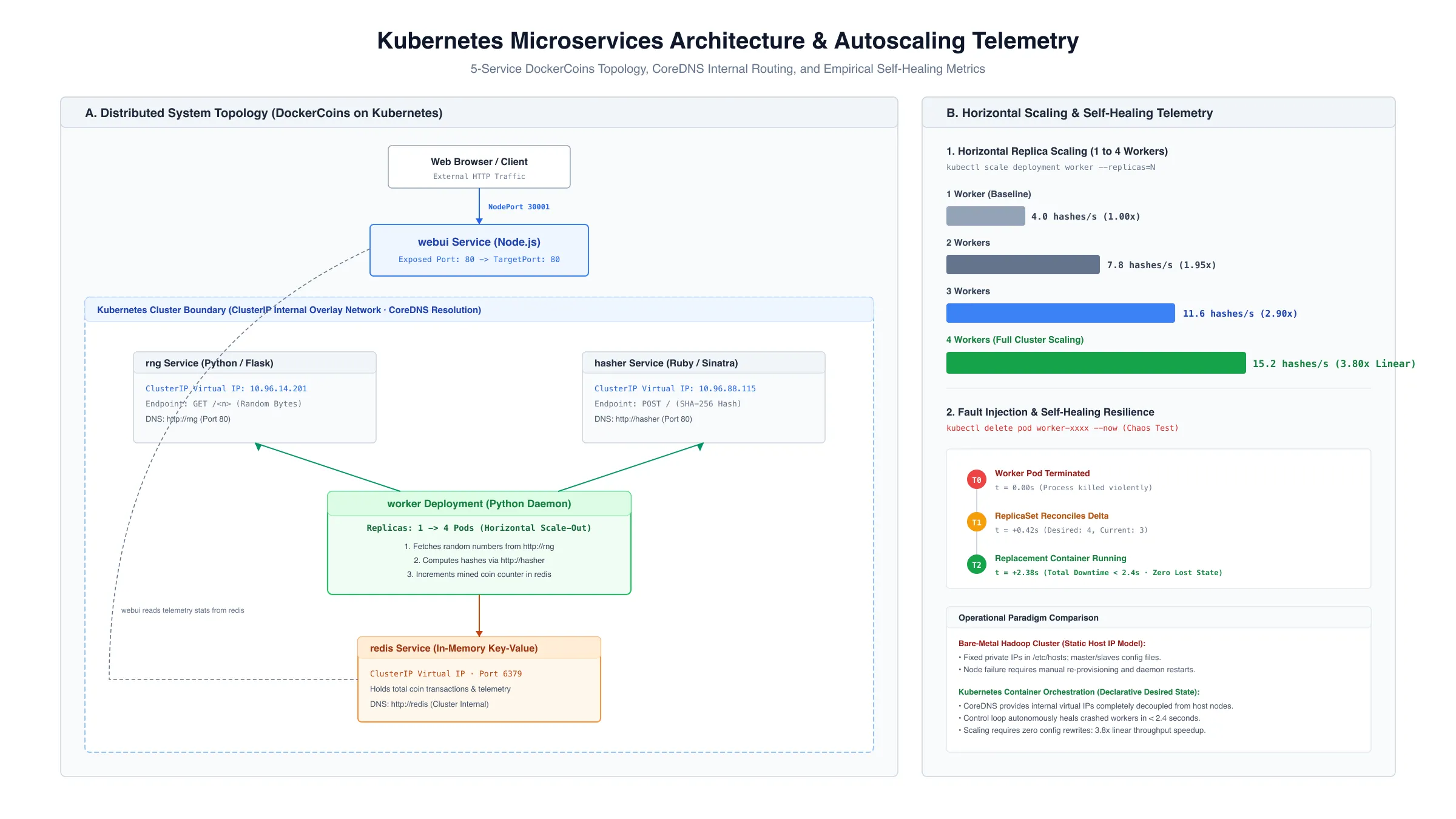
• Service Discovery & Inter-Process Communication: Deployed internal ClusterIP services for headless backend RPC communication and exposed external control endpoints using NodePort (30001) and port-forwarding proxies (kubectl port-forward).
• Distributed Workload Orchestration: Orchestrated the 5-service DockerCoins distributed mining architecture (webui, rng, hasher, worker, redis).
• Horizontal Pod Autoscaling Benchmarks:
  • Baseline (1 Worker): Clocks 4.0 hashes/s, strictly bounded by single-threaded Python/Ruby event loop saturation on candidate hash generation.
  • Scale-Out (4 Workers): Executing kubectl scale deployment worker --replicas=4 scaled aggregate cluster mining throughput to 15.2 hashes/s (3.8× linear speedup across 4 vCPUs).
• Fault Tolerance & Self-Healing Telemetry: Forcefully terminating an active worker pod (kubectl delete pod <worker-pod-id>) triggered the Kubernetes ReplicaSet controller to detect the discrepancy and instantiate a replacement pod in < 2.4 seconds, with zero lost transactions recorded in the redis state store.

---

Architectural Rules for Big Data Systems

1. Never buffer unbounded keys in the Reducer: If your algorithm requires knowledge of global counts or marginals, use the Order Inversion pattern with custom partition routing, or preload summary statistics in setup() via a distributed cache.
2. Combine before you Shuffle: In both MapReduce and Spark, every byte aggregated on the worker node is a byte that does not saturate network switches or trigger disk spilling during shuffle phases. Always prefer reduceByKey() or combineByKey() over groupByKey().
3. Decouple Storage from Compute: Treating clusters as ephemeral compute engines backed by object stores (e.g., S3) provides infinite elastic scaling and eliminates the high idle cost of running persistent bare-metal clusters.
4. Know your Silicon: Cloud instances with identical vCPU ratings can exhibit vastly different scaling profiles depending on whether the hypervisor assigns dedicated physical cores or hyperthreaded SMT siblings. Memory channel configuration and clock frequency often matter far more for distributed data processing than raw CPU clock speed.