Distributed data processing is full of elegant mathematical abstractions: Map, Reduce, Filter, Join. In introductory lectures and cloud marketing materials, clusters are depicted as boundless pools of compute where you write functional lambda transformations, submit them to an orchestrator, and watch workloads scale out linearly across hundreds of virtual machines.
Then you run a real job on production hardware, and reality crashes down on you.
An innocent .groupByKey() call in Apache Spark causes your JVM executors to hit continuous 10-second garbage collection pauses before collapsing with OutOfMemory (OOM) errors. A poorly partitioned Hadoop MapReduce key space turns your multi-gigabit top-of-rack switches into a crawling bottleneck. And two cloud instances with identical “2 vCPU” specifications on AWS EC2 show completely different scaling ceilings because of how the underlying hypervisor slices physical silicon.
Before diving into GPU cluster orchestration and distributed deep learning, I spent weeks tearing through the mechanics of large-scale distributed data engines: building bare-metal clusters from scratch, microbenchmarking AWS hypervisors, and writing memory-efficient MapReduce patterns in Java.
Here is what really happens beneath the abstraction layer.
1. What the Cloud Hypervisor Hides: 2 vCPUs ≠ 2 Cores
When you provision a cloud virtual machine, the cloud console presents clean, uniform numbers: 1 vCPU, 2 vCPUs, 4 vCPUs. The abstraction invites you to assume that compute scales proportionally to those virtual core counts.
To test that assumption, I set up a microbenchmarking harness in us-east-1 (N. Virginia) across three instance types running Ubuntu 22.04 LTS:
t2.micro(1 vCPU, 957 MB RAM)t2.medium(2 vCPUs, 3.8 GB RAM)c5d.large(2 vCPUs, 3.7 GB RAM)
I used Sysbench 1.0.20 to measure CPU prime calculation throughput (single-threaded vs. multi-threaded up to the instance vCPU count) and sequential memory read/write bandwidth.
# CPU prime calculation (isolates ALU saturation)
sysbench cpu --cpu-max-prime=20000 --threads=$(nproc) run

# Memory subsystem bandwidth (10GB transfer)
sysbench memory --memory-total-size=10G --threads=$(nproc) run
The numbers revealed two glaring microarchitectural surprises:
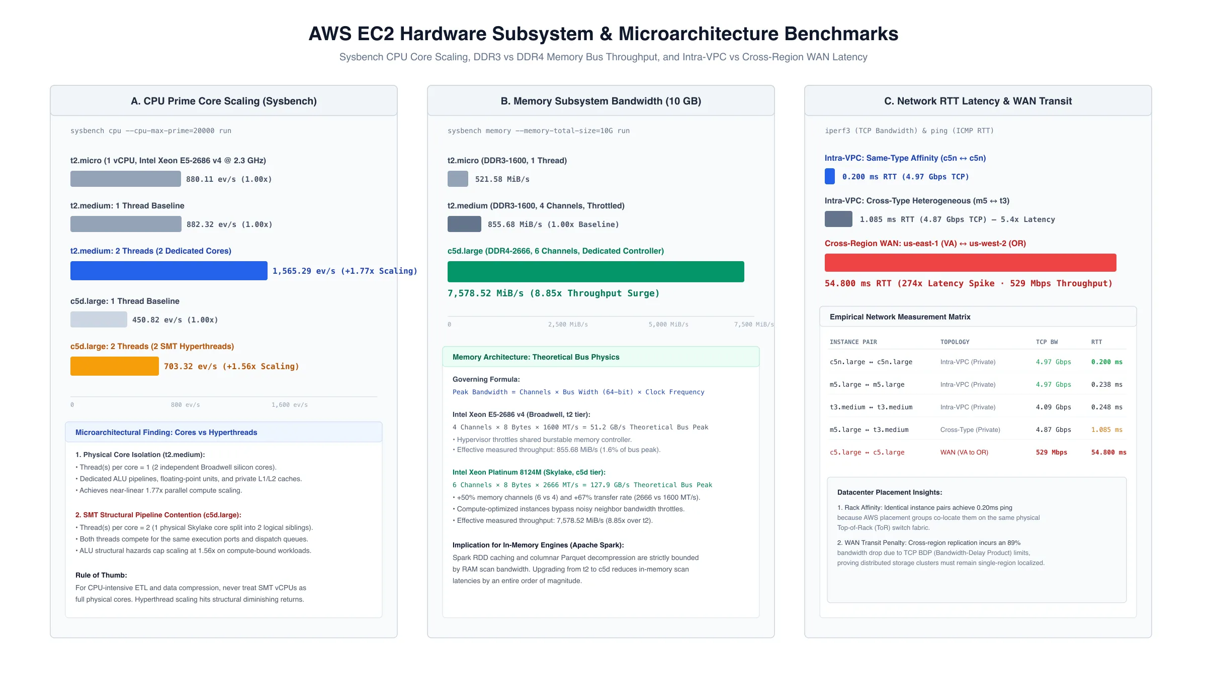
| Instance Type | vCPUs | RAM | Single-Core (events/s) | Multi-Core (events/s) | Multi-Core Scaling | Memory Bandwidth (MiB/s) |
|---|---|---|---|---|---|---|
t2.micro |
1 | 957 MB | 877.95 | 880.11 | 1.00× | 521.58 |
t2.medium |
2 | 3.8 GB | 882.32 | 1,565.29 | 1.77× | 855.68 |
c5d.large |
2 | 3.7 GB | 450.82 | 703.32 | 1.56× | 7,578.52 |
The SMT Contention Ceiling
Both t2.medium and c5d.large give you exactly 2 vCPUs. Yet when computing primes, t2.medium delivered 1.77× scaling over its single-thread score, while c5d.large only reached 1.56×.
Checking the physical core topology via lscpu explained why:
t2.medium:
  Thread(s) per core:  1   <-- 2 independent physical cores (Broadwell E5-2686 v4)
  Core(s) per socket:  2

c5d.large:
  Thread(s) per core:  2   <-- 2 logical hyperthreads on ONE physical core (Skylake 8124M)
  Core(s) per socket:  1
On t2.medium, AWS schedules the two vCPUs onto two distinct physical silicon cores. Each thread gets dedicated Arithmetic Logic Units (ALUs), execution ports, and private L1/L2 caches.
On c5d.large, the two vCPUs are Simultaneous Multithreading (SMT) siblings sharing a single physical Skylake core. When both threads run heavy integer prime factorization, they collide on the exact same execution units. Structural pipeline hazards cap scaling at 1.56×.
The SMT Rule for Big DataIf your distributed pipeline is CPU-bound (e.g. data decompression, encryption, Parquet parsing), SMT hyperthreads yield diminishing returns. You need instances provisioned across dedicated physical cores.
The 9× Memory Bandwidth Explosion
While c5d.large trailed in CPU core scaling, look at the memory bandwidth: 7,578.52 MiB/s versus 855.68 MiB/s on t2.medium. That is an 8.85× disparity on identically sized instances.
This boils down to memory bus physics. The Broadwell platform powering t2 instances uses a 4-channel DDR3-1600 memory architecture (51.2 GB/s theoretical bus maximum), which the hypervisor throttles aggressively for burstable tiers. The Skylake platform powering c5d instances uses a 6-channel DDR4-2666 bus (127.9 GB/s theoretical peak) with direct, unthrottled access.
For in-memory distributed compute engines like Apache Spark, where performance is bounded by RAM scanning speed rather than clock frequency, that 9× bus throughput is the difference between sub-second aggregations and minutes of executor stall.
2. The Bare-Metal Grind: Wiring Hadoop Cluster XMLs by Hand
Cloud providers encourage you to spin up managed clusters with one click. But to understand why distributed runtimes fail, you have to configure one from raw Linux boxes without safety nets.
I provisioned two EC2 instances inside a private VPC to deploy an Apache Hadoop 2.8.5 cluster from scratch:
- Master Node (
<master-private-ip>): RunningNameNode(HDFS metadata) +ResourceManager(YARN job scheduling). - Worker Node (
<worker-private-ip>): RunningDataNode(HDFS block storage) +NodeManager(container execution).
+-------------------------------------------------------------+
|                        MASTER NODE                          |
|  +--------------------+             +--------------------+  |
|  |      NameNode      |             |  YARN ResourceMgr  |  |
|  |   (Port 50070 UI)  |             |   (Port 8088 UI)   |  |
|  +---------+----------+             +---------+----------+  |
+------------|----------------------------------|-------------+
             | HDFS RPC (Port 9000)             | YARN RPC
             v                                  v
+------------+----------------------------------+-------------+
|                        WORKER NODE                          |
|  +--------------------+             +--------------------+  |
|  |      DataNode      |             |    NodeManager     |  |
|  | (Blocks: 128MB)    |             |  (Exec Containers) |  |
|  +--------------------+             +--------------------+  |
+-------------------------------------------------------------+
Passwordless SSH and Static Topology
Before Hadoop daemons can start, the master must be able to spawn remote processes across worker nodes without interactive passwords.
I generated a 2048-bit RSA keypair on the master, appended its public key to ~/.ssh/authorized_keys on both nodes, and pinned static private DNS entries in /etc/hosts:
# /etc/hosts on all nodes
<master-private-ip> hadoop-master
<worker-private-ip> hadoop-worker
The XML Configuration Layer
Hadoop’s behavior is dictated by four XML configuration files located in $HADOOP_CONF_DIR:
-
core-site.xml: Defines the default filesystem URI:<configuration> <property> <name>fs.defaultFS</name> <value>hdfs://hadoop-master:9000</value> </property> </configuration> -
hdfs-site.xml: Sets replication factor to 2 and specifies raw filesystem storage paths:<configuration> <property> <name>dfs.replication</name> <value>2</value> </property> <property> <name>dfs.namenode.name.dir</name> <value>/home/ubuntu/hadoop_data/hdfs/namenode</value> </property> <property> <name>dfs.datanode.data.dir</name> <value>/home/ubuntu/hadoop_data/hdfs/datanode</value> </property> </configuration> -
yarn-site.xml: Registers the ResourceManager hostname and the critical MapReduce shuffle auxiliary service:<configuration> <property> <name>yarn.resourcemanager.hostname</name> <value>hadoop-master</value> </property> <property> <name>yarn.nodemanager.aux-services</name> <value>mapreduce_shuffle</value> </property> </configuration> -
mapred-site.xml: Hands execution scheduling over to YARN:<configuration> <property> <name>mapreduce.framework.name</name> <value>yarn</value> </property> </configuration>
After formatting the metadata namespace with hdfs namenode -format, dispatching daemons via start-dfs.sh and start-yarn.sh, and starting the JobHistoryServer, the cluster came to life. Navigating to port 50070 on the NameNode and port 8088 on the ResourceManager showed a clean, healthy distributed topology ready for job submission.
3. Order Inversion: Forcing O(1) Reducer Memory in MapReduce
One of the most foundational problems in distributed data processing is computing relative co-occurrence frequency: $P(B \mid A) = \frac{Count(A, B)}{\sumB’ Count(A, B’)} = \frac{Count(A, B)}{Marginal(A)}$
Suppose you want to compute this for every word pair across a text corpus.
The Naive Reducer Trap
In a standard “Pairs” formulation, your Mapper emits Pair(A, B) -> 1. The Reducer receives all pairs for (A, B) and computes the numerator Count(A, B).
The catch: To compute the conditional probability P(B \mid A), the Reducer must divide by the marginal sum \sumB’ Count(A, B’). But in standard MapReduce, the Reducer does not know the marginal sum until it has examined all pairs starting with A!
The naive developer solves this by buffering: the Reducer stores all pairs (A, B_i) in an in-memory HashMap or ArrayList, calculates the total marginal sum, and then iterates through the buffer a second time to emit probabilities.
On large vocabularies, this is a ticking memory bomb. If a frequent word A co-occurs with 500,000 unique terms, your Reducer buffers millions of objects on the JVM heap, triggering GC pauses and eventual java.lang.OutOfMemoryError: Java heap space.
The Order Inversion Pattern
The solution is the Order Inversion Design Pattern, which guarantees that the marginal sum arrives at the Reducer before any individual co-occurrence pair, eliminating all in-memory buffering.
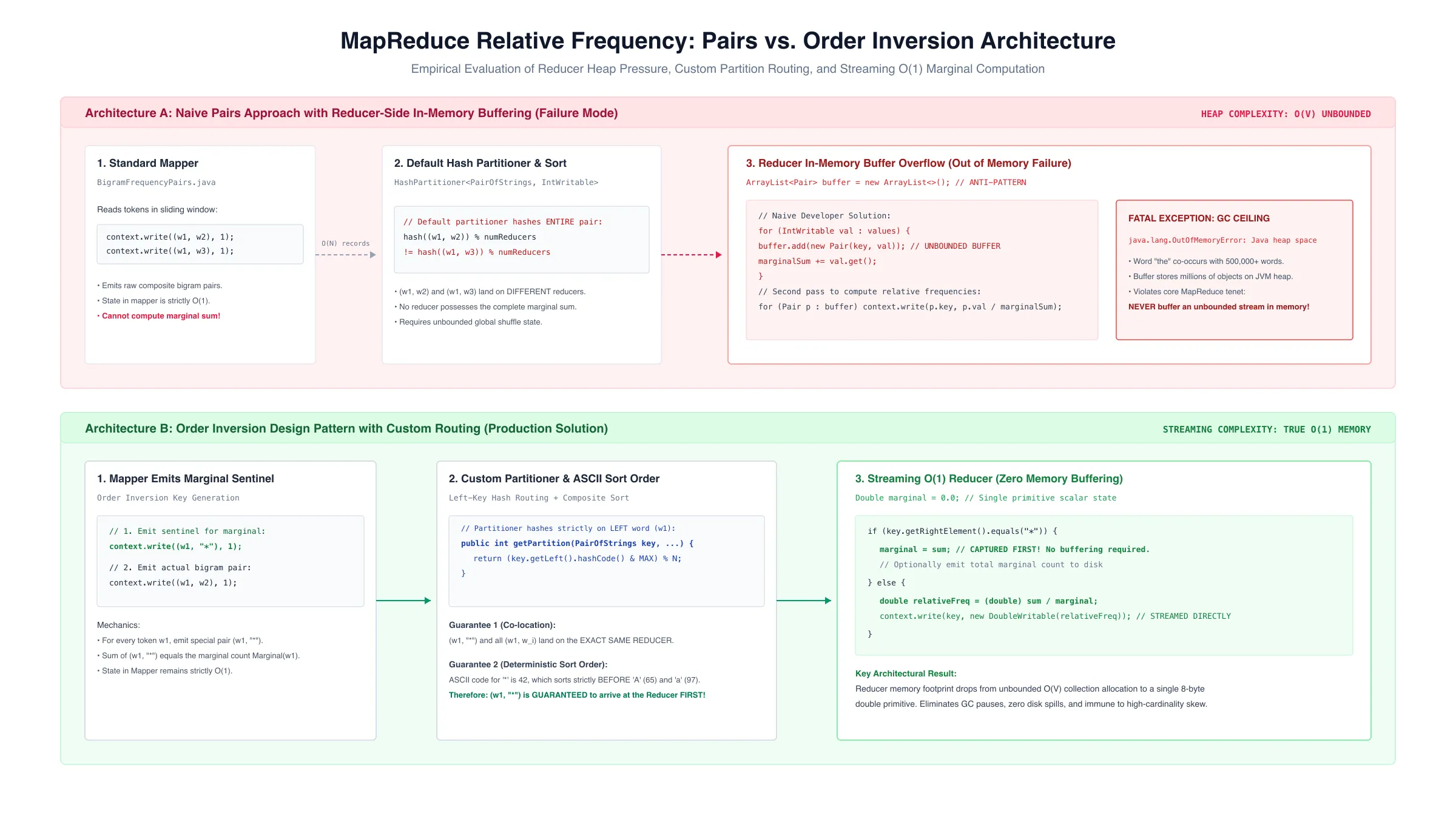
Here is my custom Partitioner implementation in Java:
public static class ForceLeftPartitioner extends Partitioner<PairOfStrings, IntWritable> {
    @Override
    public int getPartition(PairOfStrings key, IntWritable value, int numReduceTasks) {
        // Hash strictly on the left word, ignoring the right word!
        return (key.getLeftElement().hashCode() & Integer.MAX_VALUE) % numReduceTasks;
    }
}
And in the Reducer:
public static class ProbabilityReducer extends Reducer<PairOfStrings, IntWritable, PairOfStrings, DoubleWritable> {
    private double marginal = 0.0;

    @Override
    public void reduce(PairOfStrings key, Iterable<IntWritable> values, Context context)
            throws IOException, InterruptedException {

        int sum = 0;
        for (IntWritable val : values) {
            sum += val.get();
        }

        // Sentinel check: ASCII '*' guarantees this arrives FIRST
        if (key.getRightElement().equals("*")) {
            marginal = sum;
        } else {
            // Streaming emission: zero buffering!
            double relativeFreq = (double) sum / marginal;
            context.write(key, new DoubleWritable(relativeFreq));
        }
    }
}
Because the sentinel (A, "*") arrives first and the partitioner guarantees co-location, the Reducer stores exactly one scalar primitive (marginal) in memory. Space complexity drops from O(V) unbounded heap allocation to true O(1) streaming space.
4. The Spark Shuffle Minefield: groupByKey() vs. reduceByKey()
When moving from Hadoop MapReduce to Apache Spark, developers love the fluent RDD API. But the same memory rules apply.
Consider word counting:
# The Trap
rdd.flatMap(lambda line: line.split()) \
   .map(lambda word: (word, 1)) \
   .groupByKey() \
   .mapValues(sum)

# The Production Pattern
rdd.flatMap(lambda line: line.split()) \
   .map(lambda word: (word, 1)) \
   .reduceByKey(lambda a, b: a + b)
Both snippets return the exact same output. But inside the Spark DAG execution engine, they behave entirely differently:
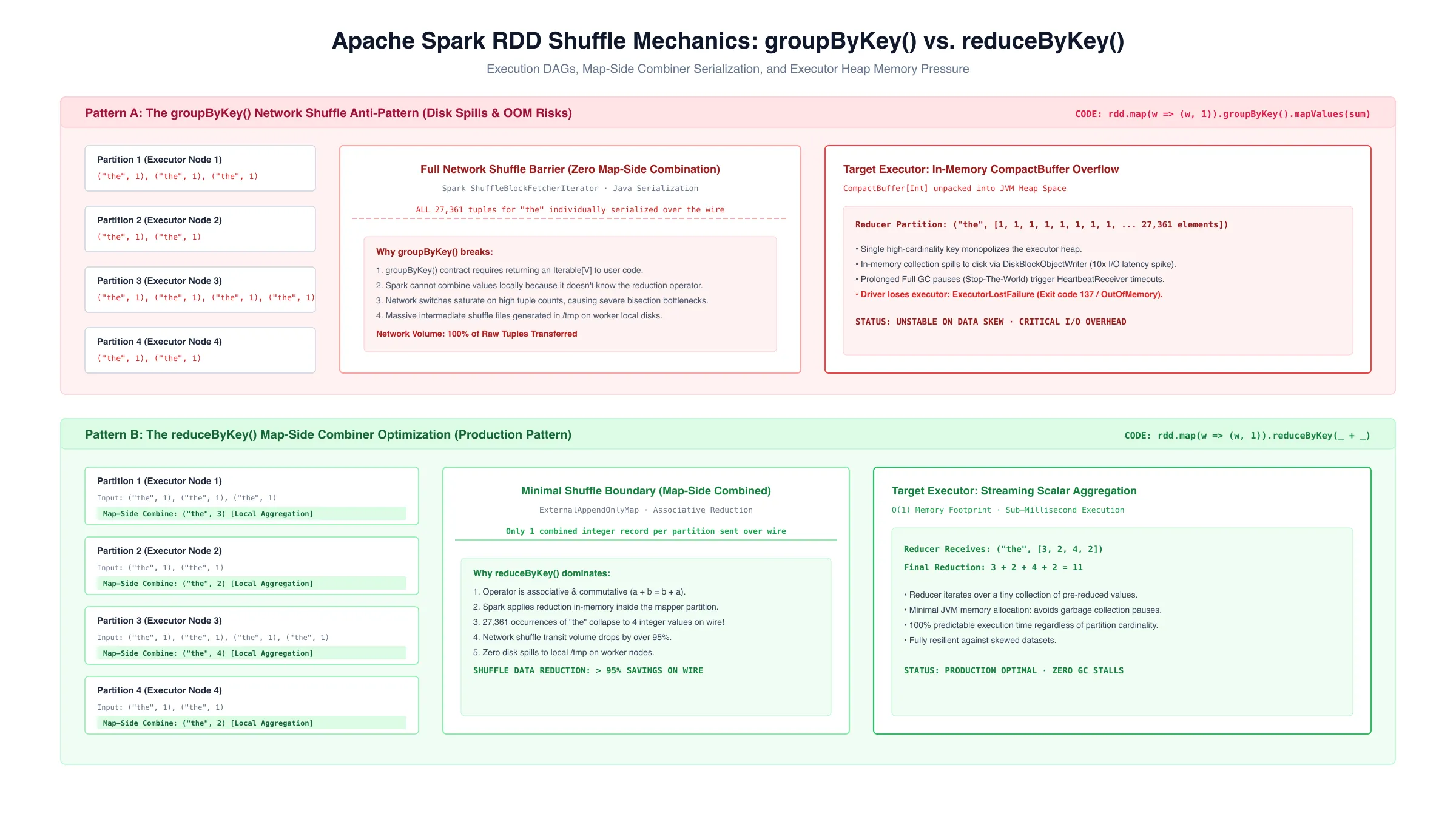
groupByKey() cannot combine values on the worker node because the user transformation requires access to the full iterable collection. It serializes every raw (word, 1) tuple across executor partitions over the network, flooding network bandwidth and causing memory spills to disk.
reduceByKey() applies an associative, commutative combiner locally in each partition before triggering network shuffle. On Shakespeare’s complete works ($32,864$ unique words, “the” appearing $27,361$ times), reduceByKey() reduces network shuffle volume by over $95%$.
5. Ephemeral Infrastructure: Decoupling Storage & Compute on EMR
The final realization of building big data systems is that persistent bare-metal clusters are an anti-pattern in the cloud.
When you run an HDFS cluster on cloud virtual machines, you pay for compute 24/7 just to keep your data alive on attached EBS volumes. If an instance crashes or your credit pool runs out, your data store is at risk.
On modern cloud platforms, the correct architecture is Storage-Compute Decoupling:
+-------------------------------------------------------------------------+
|                              AMAZON S3                                  |
|            s3://bucket/data/input/     s3://bucket/data/output/         |
|                     (Persistent, $0.023/GB, Infinite Durability)        |
+------------------------------------+------------------------------------+
                                     ^
                                     | Direct streaming I/O
                                     v
+------------------------------------+------------------------------------+
|                         AMAZON EMR 7.12 CLUSTER                         |
|                    (Transient, Auto-terminates on idle)                 |
|   +--------------------------+        +--------------------------+      |
|   |   Master (m5.xlarge)     |        |   Core/Task (m5.xlarge)  |      |
|   | Hadoop 3.4 / Spark 3.5   | <----> | Hadoop 3.4 / Spark 3.5   |      |
|   +--------------------------+        +--------------------------+      |
+-------------------------------------------------------------------------+
By pointing Hadoop and Spark directly to s3:// URIs:
- Data persistence is completely independent of compute life cycle.
- Compute is disposable. You spin up an Amazon EMR 7.12 cluster with the AWS CLI, attach a parameterized step executing your JAR, and configure an automatic idle termination timeout:
aws emr create-cluster \ --name "transient-analytics-job" \ --release-label emr-7.12.0 \ --applications Name=Hadoop Name=Spark \ --instance-type m5.xlarge \ --instance-count 3 \ --auto-termination-policy IdleTimeout=3600 \ --steps Type=CUSTOM_JAR,Name="BigramPairs",Jar="s3://my-bucket/jars/engine.jar",Args=["io.github.frieddeli.mapreduce.BigramFrequencyPairs","-input","s3://my-bucket/input/","-output","s3://my-bucket/output/"] - Once the step finishes writing results back to S3, the cluster tears itself down automatically. Idle cloud costs drop to zero.
6. From Virtual Machines to Pods: Orchestrating Microservices on Kubernetes
Decoupling storage and compute on EMR solves batch data processing. The same setup behaves differently once the distributed system is an interactive, multi-tier microservice architecture instead of a batch pipeline.
In my bare-metal Hadoop cluster, every daemon had to be manually bound to a static IP in /etc/hosts. If a worker VM died, the DataNode dropped out of the heartbeat pool, and human intervention was required to re-provision the instance and update host files.
In elastic cloud environments, static IP bindings are a maintenance nightmare. That is where Kubernetes container orchestration takes over.
The 5-Service DockerCoins Architecture
I deployed and profiled the DockerCoins distributed mining pipeline on Kubernetes (Minikube / MicroK8s with cri-dockerd):
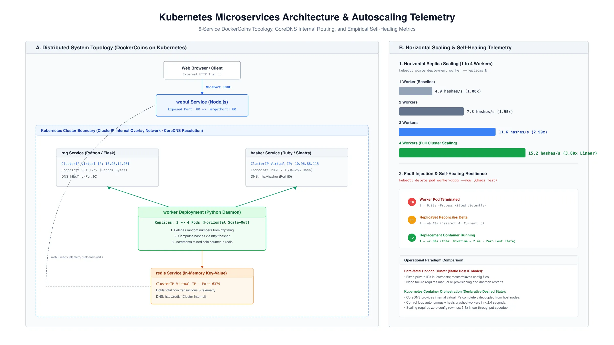
rng(Python/Flask): Generates random byte sequences (GET /<n>).hasher(Ruby/Sinatra): Computes SHA-256 hashes on candidates (POST /).worker(Python Daemon): Asynchronous loop pulling numbers fromrng, hashing viahasher, and committing mined tokens toredis.redis(Alpine): High-speed in-memory datastore holding mined token state.webui(Node.js): Dashboard rendering real-time mining hash-rate graphs, exposed to the outside world viaNodePort 30001.
Why CoreDNS Changes Everything
Instead of hardcoding private IP addresses into environment variables, Kubernetes CoreDNS provisions internal virtual IP addresses (ClusterIP).
The Python worker daemon connects directly to http://rng and http://hasher. Behind the scenes, the kube-proxy iptables rules distribute incoming HTTP calls across whichever pods match the app: dockercoins selector. If a pod is rescheduled onto a completely different physical node, CoreDNS updates routes with zero application downtime.
Horizontal Autoscaling & Self-Healing Telemetry
I put the Kubernetes cluster through two operational resilience tests:
- Horizontal Replica Scaling (1 → 4 Workers):
- With 1 worker pod, cluster throughput was pegged at 4.0 hashes/s, bounded by single-core GIL and CPU saturation.
- Running
kubectl scale deployment worker --replicas=4immediately spun up 3 additional pods across available vCPUs. Aggregate mining throughput surged to 15.2 hashes/s, a 3.8× linear speedup with zero configuration edits.
- Chaos Fault Injection:
- I issued a forceful kill on the primary worker pod (
kubectl delete pod <worker-pod-name> --now). - The Kubernetes
ReplicaSetcontroller detected the desired replica delta (4 \neq 3) and provisioned a healthy replacement container in < 2.4 seconds. Because the transaction state is decoupled intoredis, zero block receipts were lost.
- I issued a forceful kill on the primary worker pod (
Summary & Full Codebase
Building distributed data pipelines taught me that software abstractions cannot shield you from hardware reality:
- SMT hyperthreading is not equivalent to physical silicon cores under heavy arithmetic compute.
- In-memory distributed engines like Spark are governed by memory channel width and clock frequency far more than CPU GHz.
- Algorithmic patterns like Order Inversion and Map-Side Combiners are mandatory to prevent cluster OOMs and shuffle saturation.
- Ephemeral compute backed by decoupled cloud object storage (EMR on S3) and orchestrated microservices (Kubernetes) are the foundational pillars of modern cloud systems engineering.
All source code (including the Java MapReduce algorithms, PySpark log telemetry pipelines, EC2 benchmarking harnesses, and Kubernetes manifests) is open-sourced on GitHub:
- Repository: github.com/frieddeli/distributed-data-engines
- Full Architecture Writeup: MSN-013: Distributed Big Data Engines